Taking Risks and Making Decisions
I would venture that when many data scientists think of classification, they envision a figure like the one below in their heads.
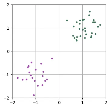
This type of depiction is ubiquitous, be it in introductory lecture slides, papers or blog posts but I often worry that it is responsible for setting unrealistic expectations for data scientists. My main concern isn’t the low-dimensional or toy-like nature of the data, but rather the perfect separability between the classes. This can lead one to believe that zero classification error is an achievable outcome in real life which is not necessarily the case. In general, one has to accept that mistakes are inevitable, even by so-called “perfect models” and that the best one can do is achieve an advantageous trade-off between different kinds of errors.
In this blog post I want to explore some of the fundamentals of decision theory which is what allows us to formalize these trade-offs and make optimal decisions.
The Classification Problem
To begin, let us formally define the standard classification problem. I will assume that data is sampled i.i.d. from an unknown joint distribution over , which I will refer to as the data generating distribution.
As a running example I will consider the distribution defined by the following simple hierarchical model:
The following figure depicts, on the left, a sample from this distribution (with ) overlaid on the input density, . On the right I plot instead some of the contour lines of , in color, over .
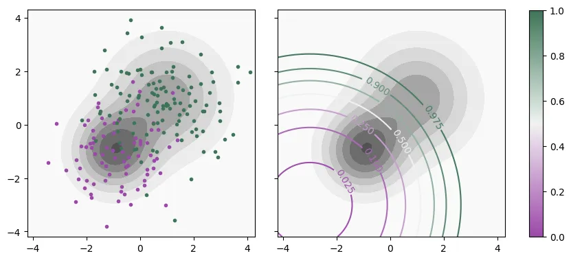
Figure 2: Contour plot of in gray overlaid by a sample from (left) and contour lines of (right).
Our objective is to assign an action to every point, , in the input space. In other words, we would like to find a mapping, from the input space to an action space . In a typical classification scenario, actions correspond to predicting one of the classes and thus we can identify . The mapping, , which I will call a classification rule, simply partitions the input space into disjoint regions
where , is the region of the input space where class is predicted.
Notice that, on the example above, no matter how we choose the , we are going to make mistakes because the supports of the two classes overlap significantly. In fact, only converges to 1 as goes to infinity (in any direction). As a result, at any point , there is a nonzero chance that we would find a sample from either class. The mistakes we can make here come in two kinds, false positives (FP) and false negatives (FN) and we would like to find a classification rule that achieves a good trade-off between the two.
Note on overfitting
A common source of confusion is that we can always fit a classifier with a wiggly enough decision boundary that perfectly classifies a sample like what we see on the left of Figure 2. Note however that what we want to accomplish is to find a classifier that performs well under the data generating distribution, not on a particular sample from it. In other words, we want a classifier that generalizes to any future set of samples drawn from . For the distribution above, we simply have to accept that such a classifier will make mistakes on this future data since the class conditional distributions overlap.
Minimizing Risks
To express our preferences regarding trade-offs we can attribute a cost (or loss) to every possible combination of the true label and prediction . For a classification problem with classes these costs can be collected into a -by- matrix with coefficients . The risk that we want to minimize can then be written as the expected loss incurred by our classification rule, , under the data generating distribution,
where the second line follows from decomposing the expectation using the chain rule of probability. For convenience we can define the inner expectation as
which is usually called the conditional risk. It is the expected cost incurred when we choose to predict at a point and it is only a function of these two quantities unlike Equation 2 which is a functional of .
To minimize with respect to , we can note is that the problem is separable over . What I mean is that it suffices to choose the action that minimizes the conditional risk pointwise for every :
If the data generating distribution, , was known, the problem would essentially be solved. For any given point , we could compute the conditional risk for every possible prediction and choose the smallest value as our prediction. This optimal classification rule for a given risk is typically called Bayes optimal and the achieved risk the Bayes error.
Binary Classification
Let us consider the simplest case of classification: binary classification. I will use the following slightly more convenient notation for the elements of the cost matrix:
The total risk can be decomposed as
where, for example,
represents the overall probability that a sample drawn from the data generating distribution is a true negative for the rule . This is not to be confused with the true negative rate (TNR) which is typically defined as the rate at which a negative example (drawn from ) is correctly classified. The two are related by , where is the base rate for the negative class. I will adopt a similar notation for the remaining outcomes (FP, FN and TP), as well as their respective rates.
The conditional risks of predicting the negative and the positive classes at a point are, respectively,
We should predict if the expected cost we incur from doing so is smaller than the expected cost for predicting 0, and vice versa. The optimal policy is therefore:
After some trivial algebraic manipulations we find that the condition to predict 1 is equivalent to
In other words, the Bayes optimal classifiers for binary classification with fixed costs correspond to a simple thresholding of . The particular threshold is determined by the costs of each possible outcome. For our example problem above, the optimal decision boundaries are those depicted on the right of Figure 2.
Trade-offs in Binary Classification
Note that, while for binary classification there are 4 possible outcomes and 4 costs that can be specified, there is only one relevant degree of freedom for the cost matrix. This is because:
- Any affine scaling of a risk functional doesn’t change the optimal policy, which means 2 degrees of freedom are irrelevant.
- The relationship eliminates another degree of freedom.
Thus, we can express the relevant trade-offs in terms of a single cost parameter, which I will choose as the threshold , as defined in Equation 3. The risk can then be equivalently (in the sense that it leads to the same Bayes optimal classifier) written as
This lets us interpret as a convex combination parameter between the probability of a false positive and a false negative, expressing the trade-off between the two. Conveniently, it is also the threshold we should choose to apply to to optimize this risk.
Below is a depiction of the FPR and FNR of every Bayes optimal classifier as we vary this cost parameter , therefore establishing a pareto front for what is achievable for this data generating distribution. I also pick two particular cost parameters ( and ) and plot the respective level sets for their achieved Bayes Errors which, as we can see, are tangent to the pareto front.
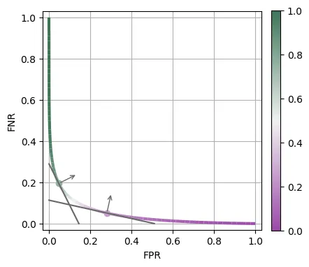
Figure 3: FPR and FNR achieved by each Bayes optimal classifier as we vary the cost parameter (color).
When Costs are a Function of Input
In the previous section we saw that when costs only depend on and the action taken, the Bayes optimal classifier corresponds to thresholding of at a fixed value. We can now ask what happens in the general case where the costs also depend on . Consider, for example, the following cost matrix:
Here we are modeling a scenario where represents the logarithm of the cost of a false negative (raised to a power of ) and a false positive has a fixed cost . The optimal condition for predicting a positive example can be found to be:
Unlike the previous case, the threshold now depends on and the decision boundaries do not strictly align with the level sets of . The figure below shows how these decision boundaries look for three different values of as we vary . The cost of a false negative increases with , which causes the optimal decision boundary to be more conservative in predicting positive for larger values of . As increases, these boundaries align more and more with the level sets of , ignoring .
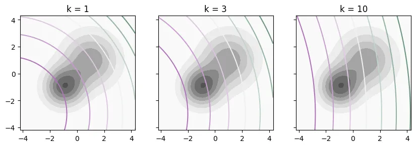
Figure 4: Bayes optimal decision boundaries as a function of (subplot) and (encoded in the color, using a different color scale for each subplot).
A General Approach
Implementing a Bayes optimal classifier requires knowledge of the data-generating distribution, specifically the true conditional distribution . In practice we need to estimate the latter by training a machine learning model, leading us to the following general approach to obtain an approximate solution to the classification problem with arbitrary costs:
- Find the solution of the decision problem (analytically) as a function of .
- Train a machine learning model to estimate .
- Use the estimated as a stand in for the real one to compute predictions.
This neatly decouples the classification problem into two steps, only one of which requires statistical inference.

You might be wondering how we can go about step 2. In particular, how do we guarantee that a machine learning model learns to estimate ? I will reassure you that that is probably already the case for your model of choice if it is trained to minimize a strictly proper loss like log loss (also known as cross-entropy). This typically includes deep learning models, as well as other classical models like XGBoost and Random Forests.
In fact, A strictly proper loss can be interpreted as a weighted mixture of all possible classification risks with different cost parameters, (more about that in a future blog post). Intuitively, training a discriminative model with such a loss is equivalent to simultaneously fitting classifiers for every possible value of . Afterwards, we just need to choose the right one for our particular problem by using our desired value of as a threshold.
Note that I am not claiming that this proposed approach is optimal in any sense. In fact, training a classifier directly end to end on the desired risk functional (instead of a mixture of many risks) should be more sample efficient. But that approach is impractical since classification risks are typically discontinuous functions of model parameters and hard to optimize, unlike smooth proper losses like the log loss. Furthermore, the proposed approach should still be consistent: if the model is consistent (i.e., converges to the true conditional distribution as the number of training points increases), so should the “plug in” decision boundary derived from it.
A Real World Example
To illustrate how the theory outlined above applies in a practical setting, I ran a simple experiment on the Taiwan Credit Dataset. The goal on this dataset is to predict the default of credit card clients and for this I trained a XGBoost binary classification model using 80% of the data.
Training details
I used cross-validation to manually tune only the most important hyperparameters (learning rate, number of boosting rounds and number of leaves per tree), in order to minimize log loss, using a further 80%/20% train/validation split of the full training data (80% of the full dataset).
After picking acceptable values for these hyperparameters, I then retrained the model on the full training set.
This final model was trained for 706 boosting rounds with a learning rate of 0.0075 and 32 leaves per tree (using a lossguide policy).
On the left panel of the figure below I plotted the trade-off curve computed on the remaining 20% of held-out data when considering classification rules obtained by directly thresholding the model’s predictions (note, that this is essentially a ROC curve inverted along the y-axis). Since we are relying on an estimate of , the classification rules we obtain are not necessarily Bayes optimal (as in Figure 3). However, if the model is good enough, they are hopefully a reasonable approximation.
I also picked two particular thresholds (0.1 and 0.25) and marked these points on the curve with a circle marker, together with the level sets of the risks that they supposedly minimize (plotted as straight lines). We can see that, in practice, these are not the threshold values that minimize the respective risks as predicted by the theory (those, I plotted with a star marker). They are, however, relatively close. In particular, both theoretical thresholds achieve very similar risk values as the practical minimizers. Again, this small “deviation” from the theory is purely due to relying on an estimate of provided by a model.
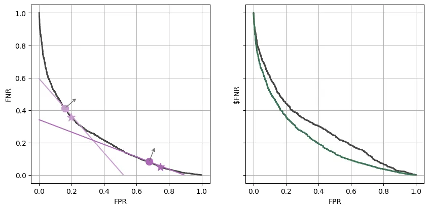
Figure 6: (left) Trade-offs achieved by plug-in classifiers in a fixed cost scenario. (right) Trade-offs achieved in the varying cost scenario for a direct thresholding of (dark gray) and the correct plug-in classifiers (green).
Let us now assume that we are trying to decide whether to approve or not a credit request. As an interesting exercise, I will consider that the cost we incur on a false negative (where we predict that the customer will not default but they do) is the total amount of credit given (in NT dollars). Conversely, I will consider the simplified scenario that a false positive only incurs a fixed cost .
In this scenario, we are interested in a trade-off between the number of false positives (since they all incur the same cost ) and the total dollar amount of credit provided to false negatives. I will denote by $FNR the total fraction of the credit requested by defaulting clients that ends up being approved as a rescaled version of this metric. If we plot the trade-offs between these two quantities when we use the classifiers obtained by thresholding we obtain the curve in dark gray on the right side of Figure 6. If instead we plot the plug in classifiers that we obtain using decision theory, as we vary the fixed cost , we get the trade-off curve in green instead. As we can see, it dominates the “naive” approach achieving quite drastic reductions in $FNR for the same FPRs.
Key Takeaway: Some data scientists may default to thresholding a machine learning model’s output to obtain a class prediction when presented with a classification problem, regardless of the cost structure. The fact that, in a binary classification problem with fixed costs, this is indeed the right thing to do only contributes to the general lack of awareness of decision theory. As we saw above, this oblivious approach can lead to very suboptimal results in scenarios with more complex costs.
Multiclass Classification
In the previous section we saw how a naive approach to binary classification, oblivious to decision theory, could yield suboptimal results in the case of input dependent costs. It turns out that for multiclass classification, the same can happen even in the case of fixed costs!
For convenience, we restate again the optimal classification rule for a classification problem:
If we are trying to minimize misclassification error (or conversely maximize accuracy), this corresponds to choosing , where denotes the Kronecker delta. In this case, the Bayes optimal classifier is then:
In other words, we should just pick the most likely class. This is the classification rule data scientists would typically default to in multi-class classification.
Balanced Accuracy
The dogma of not relying on accuracy, particularly in scenarios with unbalanced classes, is often drilled into data scientists’ heads. Many other metrics are often preferred when it comes to multiclass classification. Balanced accuracy is one of the simplest, averaging the accuracy obtained per class so as to not allow outsized influence on the evaluation metric from more prevalent classes. This is equivalent to regular accuracy, computed on a reweighed dataset where class weights are introduced to make the classes balanced. Up to an irrelevant multiplicative factor, balanced error can therefore be expressed through the following cost matrix:
where represents the original prevalence of class .
Balanced accuracy is maximized when the above balanced error is minimized. The Bayes optimal classifier is then easily found to be:
where I dropped the first term inside the argmin since it doesn’t depend on and is thus irrelevant to the minimization. Note that we end up with the extra factor which means that we should favor predicting lower prevalence classes compared to when we are trying to optimize regular accuracy.
Another Real World Example
Again, let’s check the impact of the decision rule in practice on the Covertype dataset. This dataset has 7 classes and is imbalanced with the least prevalent class corresponding to only 0.5% of the data and the largest to 49%. I trained a XGBoost multiclass classification model on 80% of the data.
Training details
Similar to the Taiwan credit dataset above, I used cross-validation to manually tune only the most important hyperparameters (learning rate, number of boosting rounds and number of leaves per tree), in order to minimize log loss, using a further 80%/20% train/validation split of the full training data.
After picking acceptable values for these hyperparameters, I then retrained the model on the full training set.
The final model was trained using 200 boosting rounds and a learning rate of 0.25 and 512 leaves per tree (using a lossguide policy).
In the table below, I report the accuracy and balanced accuracy obtained on the remaining 20% for this model when using the optimal decision rule derived for each respective metric.
| Decision Rule \ Metric | Accuracy | Balanced Accuracy |
|---|---|---|
| Accuracy | 97.22 | 94.45 |
| Balanced Accuracy | 97.12 | 96.12 |
As can be seen, the best results for accuracy are obtained when using the optimal decision rule for accuracy (i.e., selecting the most likely class according to the model as our prediction). Conversely, using the optimal decision rule for balanced accuracy (which takes into account an estimate of the class priors on the training set) we obtain a reasonable boost in balanced accuracy at the cost of a small decrease in accuracy. I will stress that these results are all obtained using the same model; the only change is how we generate predictions from the probabilities estimated by the model.
Conclusion
Decision theory is at the core of machine learning. It represents, for example, a sizable portion of the first chapter of Christopher Bishop’s Machine Learning book (which I highly recommend). Despite this, I find that many practicing data scientists tend to be too focused on models and forget to think about how they should be making decisions given those models. As we saw in this blog post, this can easily lead to subpar results given one’s actual business goals even on very simple decision problems.
When presented with any problem I always find it helpful to ask myself what would be the Bayes optimal solution if I had access to whatever data generating distribution. Then it is a matter of figuring out how to best approximate that solution given the practical tools at one’s disposal.
In future blog posts I intend to explore some related topics such as proper scoring rules and a different approach to approximating Bayes optimal classifiers through aligning the loss we use to train a model more directly with the risk we are trying to minimize. I will also touch on some of the pitfalls that can come from the use of common methods to “deal” with imbalanced data.